A custom model fitting using Tensoflow 2
February 29, 2020
In a a previous post, I have created a model for time series prediction with specific business rules. In a follow-up post, I have build an sklearn Estimator in order for this model to be used within the sklearn API. Here, I will demonstrate how to implement the same model using Tensorflow and its gradient descent fitting mtethod.
The model
Linear trend + seasonality modeled with Fourier series:
\[Y = \alpha X + \beta + \sum_{i=1}^{n+1}\left[ \mu_i cos(\frac{2 \pi i}{p} X ) + \nu_i sin(\frac{2 \pi i}{p} X ) \right]\]The model has $2n+2$ parameters:
- $\alpha$
- $\beta$
- $\nu_i$ and $n$ $\mu_i$ (
i = 1... n+1)
And two hyperparameters:
- $p$ and $n$
Implementation
Model
Want to see the code? Here we go. It is implemented as a single class holding:
- Hyperparameters (n and p).
- Parameters (alpha, beta, nu and mu). Since the number of paramters for the seasonal component depends on the hyperparameter n, they are initialized with a for loop.
- The model implementation (the
__call__method actually performs the prediction based on the current parameter values) - The loss function to be used for training.
- Methods to train the model, themselves having several parameters:
- the X and Y data
- the learning rate,
lr - the number of epochs,
epochs
class Model:
    """Class to hold our model implementation and fitting using TensorFlow
    """

    def __init__(self, p=52, n=6, loss_function=mse_loss):
        """Time series model

        :param p: seasonality parameters
        :param n: number of seasonal components
        :param loss_function: loss function
        """
        self.loss_function = loss_function

        # model hyperparameters
        self.p = p
        self.n = n

        # model parameters
        self.alpha = tf.Variable(-0.1, dtype="float32")
        self.beta = tf.Variable(0.1, dtype="float32")
        self.params = [
              self.alpha, self.beta,
        ]
        # the number of parameters for the seasonal component
        # is 2*n where n is the model hyperparameter
        for i in range(0, self.n):
            setattr(self, f"mu{i+1}", tf.Variable(0.1, dtype="float32"))
            setattr(self, f"nu{i+1}", tf.Variable(0.1, dtype="float32"))
            self.params.append(getattr(self, f"mu{i+1}"))
            self.params.append(getattr(self, f"nu{i+1}"))


    def _seasonal_component(self, X):
        """Compute seasonal component based
        on a Fourier serie
        """
        res = tf.zeros(len(X))
        for i in range(0, self.n):
            mu = getattr(self, f"mu{i+1}")
            nu = getattr(self, f"nu{i+1}")
            w = 2 * tf.constant(math.pi) * (i+1) / float(self.p)
            res += mu * tf.cos(w * X) + nu * tf.sin(w * X)
        return res

    def __call__(self, X):
        """Compute predictions based on linear trend + seasonal component
        """
        return self.alpha * X + self.beta + self._seasonal_component(X)

    def __repr__(self):
        params = ', '.join([str(p.numpy()) for p in self.params])
        return (
            "<Model \n\t"
            f"params=[{params}]"
            " >"
        )

    def _train_epoch(self, X, Y, lr):
        """Gradient descent training for a single epoch

        :param tf.Tensor X: training features (scaled)
        :param tf.Tensor Y: training target
        :param float lr: learning rate
        """
        with tf.GradientTape() as t:
            # predictions based on current parameters
            pred = self(X)
            # compute loss
            current_loss = self.loss_function(pred, Y)  # this is our custom loss
            # compute gradients and update parameters
            delta = t.gradient(
                current_loss, self.params
            )
            for p, d in zip(self.params, delta):
              p.assign_sub(lr * d)
        return current_loss

    def train(self, X, Y, lr=0.12, epochs=100):
        """Gradient descent training for `epochs` epoch

        :param tf.Tensor X: training features (scaled)
        :param tf.Tensor Y: training target
        :param float lr: learning rate
        :param int epochs: number of epochs
        """
        losses = []
        for epoch_count in range(epochs):
            real_loss = self._train_epoch(X, Y, lr=lr)
            losses.append(real_loss.numpy())

            if epoch_count < 10 or epoch_count % int(epochs / 20) == 0:
                print(f"Epoch count {epoch_count}: Loss value: {real_loss.numpy()}")
        return losses
Let’s talk a few minutes about the loss function.
Loss functions
Commonly used loss functions include for instance the Mean Square Error (MSE). However, in our problem, we have a custom definition for the loss, since if the dealer buys too much, he can still sell the leftover, even if it has to be at a lower price. We can then implement a custom loss, as illutrated below, and use it in the training phase of our model to find the paramter set optimizing this custom loss.
Compared to our previous numpy/scipy implementation, only the v_lossses and custom_loss functions need to be updated to operated on tensors rather than numpy arrays:
def v_losses(output, target):
  return (PURCHASSED_PRICE * output
        - tf.where(tf.less(output, target), _no_leftovers(output, target), _leftovers(output, target))
  )


def custom_loss(output, target):
  return tf.reduce_sum(v_losses(output, target)) / 1000


def mse_loss(y, pred):
    return tf.reduce_mean(tf.square(y - pred))
Results
After scaling X and Y, we can train this model with:
model = Model(p=52. / len(X), n=8, loss_function=custom_loss)
losses = model.train(X_train, Y_train, lr=0.1, epochs=1200)
Impact of the loss function
The first test I performed here, which could have been done with the scipy model as well, is to check the influence of the custom loss function on the results. For this, I only use the trend component, which is equivalent to setting n=0 in the model. The comparison of the result if illustrated below:
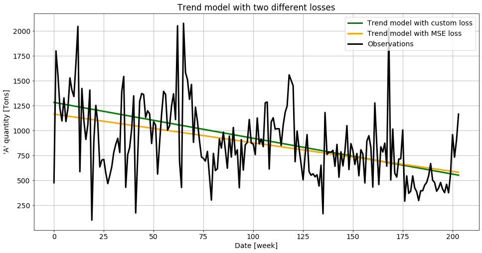
It is kind of expected that the custom loss function allows higher predictions, since the leftovers won’t be simply lost but also bring value, compared to the classical MSE loss that only sees predictions lower than the true value the same way as predictions below the true value.
Full model
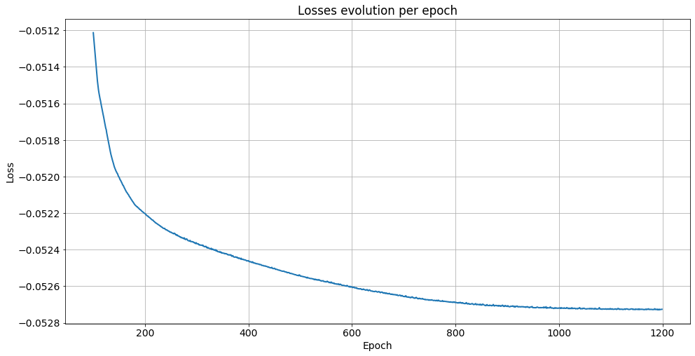
Training the full model with n=8 like in our previous implementation, we obtain this nice behaviour for the loss function:
And a final model very close to the one obtained with scipy:
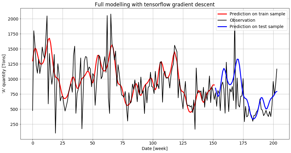
A nice advantage of tensorflow gradient descent compared to other optimization techniques, at least for this particular model, is that it is much less sensitive to the parameters initial values. Initializing all parameteres to 0 will still converge, which was not the case for the other techniques tested earlier.