A time series model
January 29, 2020
The problem
The problem can be formulated in the following way:
- a dealer buys a fresh product called A at the price of 1.5 €/ton
- the products bought on given week w are sold at the price of 2.5 €/T
- all fresh products bought during week w and that not be sold during that week are frozen to be sold the following weeks, but at the lower price of 0.8 €/T
- dealer is aware that if the demand is higher than the offer, he might loose clients, so he is very concerned to be able to meet the demand as much as possible
The goal is to predict how much the dealer should buy, to maximize the benefits (minimize the losses).
Data
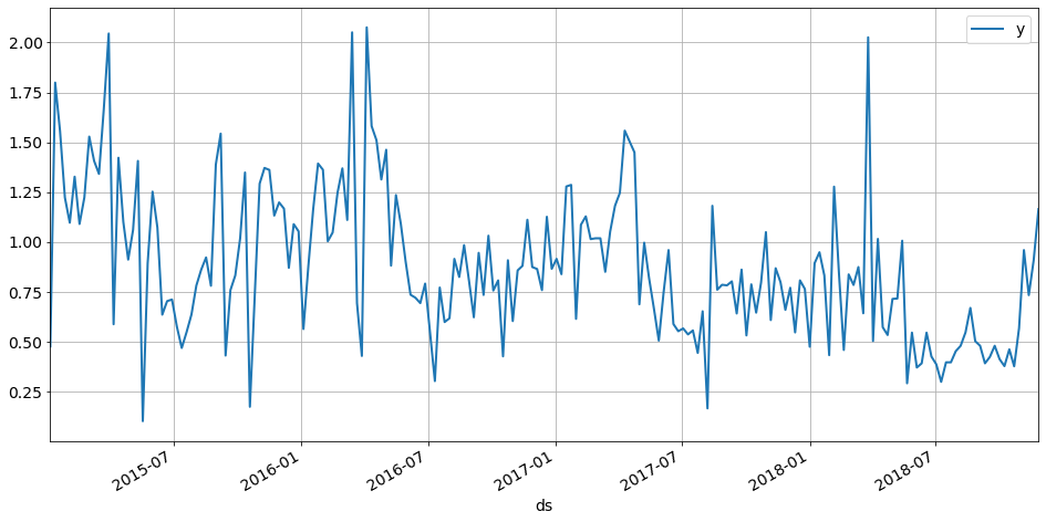
A sample data looks like:
         	ds 	y
0 	2015-01-05 	0.476
1 	2015-01-12 	1.799
2 	2015-01-19 	1.555
3 	2015-01-26 	1.222
4 	2015-02-02 	1.096
Where ds is the first day of the week and y is the number of tons of product A sold by the dealer.
Proposed solution
The proposed solution relied on scipy and a loss function computing the losses of the dealer if he buys too much product on a given day (since the left-over will be sold very cheap as frozen product). The first step was to implement a simple linear model taking into account only the evolution trend.
Trend model
To build the trend model, the first step was to write and test the loss function, since this is the quantity we will try to minimize.
PURCHASSED_PRICE = 1.5
FRESH_PRICE = 2.5
FROZEN_PRICE = 0.8
PENALTY = 0

def fresh_price(volume):
    return volume * FRESH_PRICE

def frozen_price(volume):
    return volume * FROZEN_PRICE

def loss_(y_obs, y_pred):
    """Compute the dealer gain

    :param float y_obs: real sales
    :param float y_pred: predicted sales = purchasses
    """
    expenses = y_pred * PURCHASSED_PRICE
    # if real sales are above the predicted ones
    # the only gain is the stock price, so y_pred
    if y_obs >= y_pred:
        return expenses + PENALTY - fresh_price(y_pred)
    # if real sales are below the predicted ones
    # we earn the fresh price for the sales of the day + frozen price of the leftover
    return expenses - ( fresh_price(y_obs) + frozen_price( y_pred - y_obs))

loss = np.vectorize(loss_)
The PENALTY paramter was introduced in order to penalize the dealer if he is not able to meet the customer demand. For now it is set to 0 but it can be tuned to match the dealer expectations.
The loss function is tested since it is the core of the analysis:
# make sure there is no bug in the loss function, this is the core of the analysis
def test_losses():
    b = loss([10, 10], [20, 20])
    e = ( (20 * PURCHASSED_PRICE) - 10 * FRESH_PRICE - 10 * FROZEN_PRICE)
    e = np.array([e, e])
    assert np.allclose(b, e)

    b = loss([20, 20], [10, 10])
    e = ( (10 * PURCHASSED_PRICE) + PENALTY - 10 * FRESH_PRICE)
    e = np.array([e, e])
    assert np.allclose(b, e)

test_losses()
Once we have the function we want to minimize, we still need to create the “model”. In a linear model, it is simply a function of two paramters that can be written;
def trend_model(t, params):
    """Model

    :param np.array t: times for which we want to predict the optimum purchasses
    :param np.array params: model parameters
    """
    a, b = params
    return a * t + b
Before going to the next step, the fit, we still need to split our dataset into a train and a test sample. To keep it simple, we will use the last year as test sample.
data_train, data_test = data[:len(data)-52], data[len(data)-52:]
Fit
The fit is performed using the scipy.optimize module. We first need to define the function to minimize with parameters consistent with the scipy API:
def f(params, *args):
    """Function to minimize = losses for the dealer

    :param args: must contains in that order:
    - data to be fitted (pd.Series)
    - model (function)
    """
    data = args[0]
    model = args[1]
    t = data.t
    y_obs = data.y
    y_pred = model(t, params)
    gl = loss(y_obs, y_pred)
    l = gl.sum()
    return l
Then, we can proceed to the fit, using realistic initial parameters:
tol = 500
x0 = (-6, 1.3)

ARGS = (data_train, trend_model)

res_trend = optimize.minimize(f,
                              args=ARGS,
                              x0=x0,
                              tol=tol,
                              #options={"eps": 1e-10, "maxiter": 10000}
)
Visualizing the result
The results are visualized thanks to the following code, and the resulting figure is shown below.
y_pred_train = trend_model(data_train.index.values, res_trend.x)
y_pred_test = trend_model(data_test.index.values, res_trend.x)

plt.plot(data_train.ds, y_pred_train, color="red", linewidth=3, label="Prediction on train sample")
plt.plot(data.ds, data.y, 'k-', label="Observation")
plt.plot(data_test.ds, y_pred_test, color="blue", linewidth=3, label="Prediction on test sample")
plt.xlabel("Date")
plt.ylabel("'A' quantity [Tons]")
plt.legend(loc="upper right")
plt.title("Trend modelling")
plt.show()
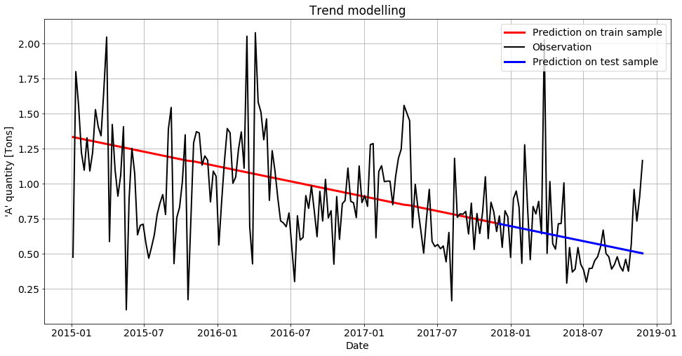
Results seem reasonable so far. Let’s first go towards a more realistic model before measuring the performances.
Adding seasonal effects
It is quite obvious from the plot that the trend is not enough to model this phenomenon, as in many times series. In this section, we implemennt seasonal effects based on a fourier series:
def fourier_series(t, p=365.25, n=10):
    """

    :pram t: times
    :pram p: seasonality period. p=365.25 for yearly, p=7 for weekly seaonality
    :param n: number of terms in the fourrier serie
    """
    x = 2 * np.pi * np.arange(1, n + 1) / p
    x = x * t[:, None]
    x = np.concatenate((np.cos(x), np.sin(x)), axis=1)
    return x


N_COMPONENT_YEARLY = 6

def seasonality_model(t, params):
    p = 52
    x = fourier_series(t, p, N_COMPONENT_YEARLY)
    return x @ params


def full_model(t, params):
    trend = trend_model(t, params[:2])
    yearly_seasonality = seasonality_model(t, params[2:N_COMPONENT_YEARLY*2+2])
    return trend + yearly_seasonality
The fit can then be performed as in the previous section:
trend_param_init = res_trend.x.tolist()
yearly_param_init = [0.1, 0.1] * N_COMPONENT_YEARLY
param_init = trend_param_init + yearly_param_init
res = optimize.minimize(f, args=(data_train, full_model),
x0=param_init,
tol = 100,
)
if res.success:
print("Fitted parameters ;", res.x)
print("Loss function value:", res.fun)
else:
print(res.message)
print(res.x)
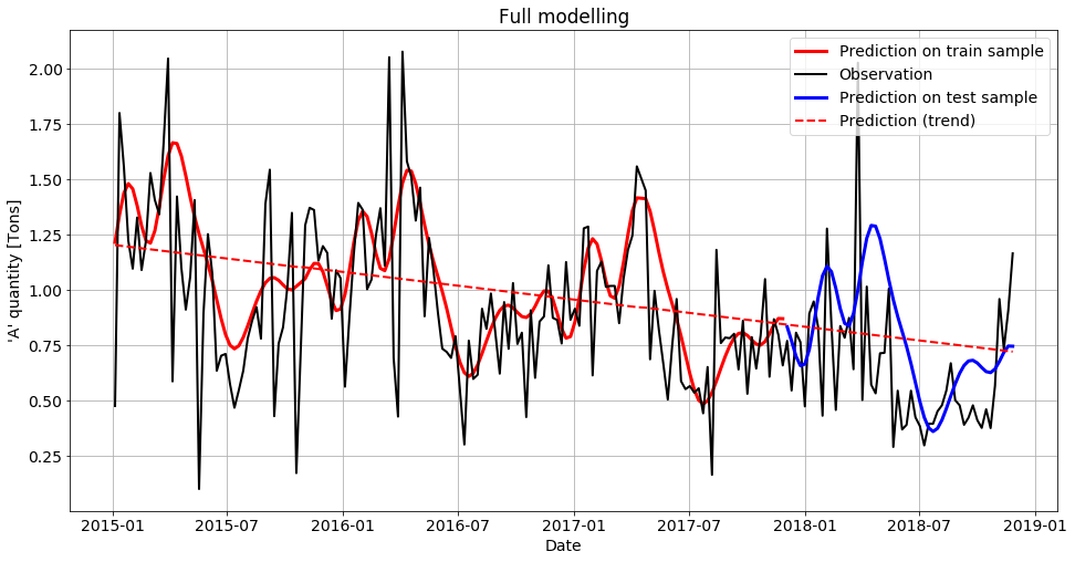
params_fit = res.x
y_pred_train = full_model(data_train.index.values, res.x)
y_pred_test = full_model(data_test.index.values, res.x)
y_pred_trend = trend_model(data.index.values, res.x[:2])
plt.plot(data_train.ds, y_pred_train, color="red", linewidth=3, label="Prediction on train sample")
plt.plot(data.ds, data.y, 'k-', label="Observation")
plt.plot(data_test.ds, y_pred_test, color="blue", linewidth=3, label="Prediction on test sample")
plt.plot(data.ds, y_pred_trend, color="red", linewidth=2, linestyle="--", label="Prediction (trend)")
plt.xlabel("Date")
plt.ylabel("'A' quantity [Tons]")
plt.legend(loc="upper right")
plt.title("Full modelling")
plt.show()
Finally, here is the result of the model:
Analyzing results
def demand_score(y_obs, y_pred):
    """Computes how often the offer was enough to satisfy the at least 90% of the demand
    """
    return ((y_obs - y_pred) / y_obs < 0.1).sum() / len(y_obs) * 100

npr = demand_score(data_test.y, y_pred_test)

print(f"The dealer will be able to deliver at least 90% of the request in {npr:.1f}% of the cases")
With our model, the dealer will be able to meet at leat 90% of the demand in 75% of the cases (3 out of 4 weeks).
We can improve this by changing the PENALTY coeffficient. For isntance, a penalty of 0.1 leads to a demand score of 86%, with a total benefit of 110 compared to 118.
Final words
This is a simple model used mainly for testing scipy and some understanding of fourier series and time series. Many things can and should be improved to use this model in real life:
- The number of components in the seasonal model is set arbitrarily. We can also think about adding different frequancies (monthly effects?).
- There is absolutely no outlier detection in this model: are the peaks we observe outliers or special events that should also be modelled?
- For this you can check the Prophet package released by Facebook for time series analysis
- etc…