Random forest VS Gradient boosting
April 03, 2020
Today I am trying to explain the difference between two ensemble models: random forest, a particular case of bagging, and gradient boosting.
Personal context: in a recent interview, among other stuffs, I was asked the difference between random forest and gradient boosting. I was not able to give a convincing answer and totally failed at this interview (not only because of that question of course, but it was so frustrating for me because I knew the answer and was just not able to put the words in the correct order :()
But, since I don’t like to repeat the same mistake twice and I think a failure is a failure only if we do not learn from it, I decided to rework that particular point, so that I never have such as confusing speech about it in the future. So this post is mainly a note to myself, but if it can useful to others, that’s even better. Please take a look at the references at the end of this article to get deeper.
Both of them are based on a “weak learner” (aka “base models”). The base models can be a decision tree, but not only. Ensemble methods consist in training multiple weak learners and somehow merge their results to build a “strong learner”. They differ on two key points:
- the way the training sets for each base model are defined
- the order in which the weak learners are trained
For a change, let me start with a summary table:
| Model | Random Forest | Gradient Boosting |
|---|---|---|
| Training data | Random sample from the full training set | Weighted training set |
| Training order | Parallel | Serial |
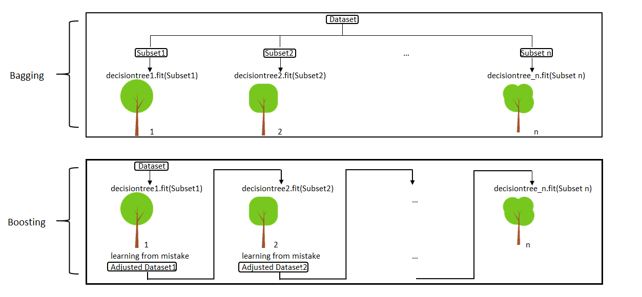
And an image (source: Basic Ensemble Learning - Step by Step Explained):
Detailed explanations coming with the following headers:
Random Forest (bagging)
Random forest creates random train samples from the full training set based on a random selection of both rows (observations) and columns (features). This is achieved thanks to a statistical technique called bootstrapping, which also gives its name to the bagging methods: Bootstrap Aggregating. Note that an interesting consequence of this way of doing is the good performance of bagging techniques in missing data handling.
A weak learner is then trained in parallel on each of the derived training sets.
Once all the models are trained, results are aggregated at the end. For a classification problem, one can use the majority-vote rule, that will classify a given observation into the class that was predicted by most of the weak learners. For a regression problem, we can use the average value of each weak learners.
Gradient boosting
Boosting ensemble methods consist in fitting several weak learners sequentially, where, at each iteration, more weight is added to the observations with the worst prediction from the previous iteration. The idea is to try and improve the results of the previous model at each iteration, focusing on the observations that were more far away from the truth.
Since each weak learner is built upon the results from the preceeding one, the computation can not be paralellized (apart from parallelism in each weak learner) and the computation can be longer.
In order to understand when to use which ensemble method, we have to understand another important concept in machine learning: bias and variance.
Bias and variance
Bias
Bias is the average distance between the expected (true) value and the predicted value. For a regression algorithm, this is the mean square error:
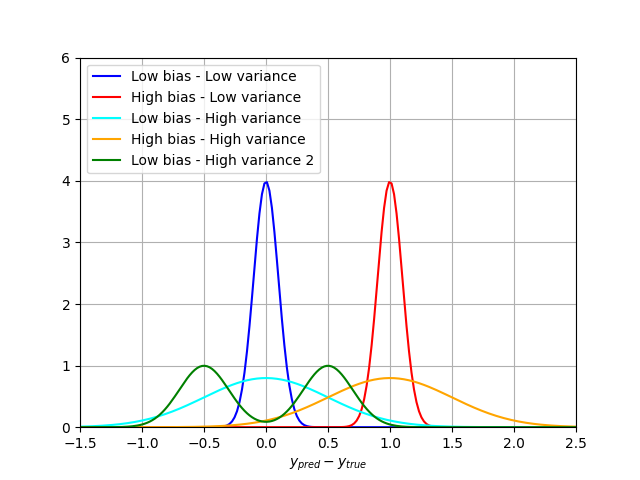
\[\mu = \frac{1}{N_{val} \sum_{i \in val} (y_i^{pred} - y_{i}^{true}) ^ 2\]The closer the bias is to zero, the more accurate the model is. If we draw the error repartition (ypred - ytrue), a very accurate model with small bias will be centered around 0, while a highly biased model will have a shifted peak. Here is an illustration of two models outputs and bias estimation:
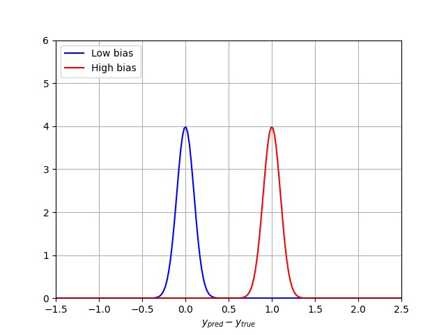
The blue curve is centered around 0 and has a low bias. On the other hand, the red curve’s average value is around 1, which means it has a high bias. In machine learning, high bias is associated to the concept of underfitting, for instance when your algorithm does not have enough data to learn, or your model does not take into account important explanatory variables.
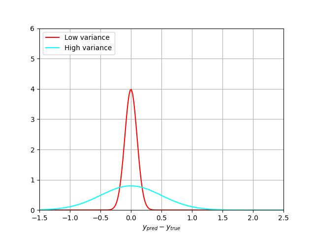
Variance
But bias is not enough to quantify the quality of a model. The bias can be small, but with a huge spread of the results. This spread is quantified with the variance, or width of the error distribution. With a low bias, we can have more or less large error distributions:
It can be even worse if the error distribution is not gaussian:
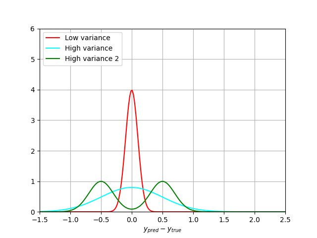
The green curve here also has a 0 bias, but higher variance.
Putting it all together on the following plot:
A fancier illustration of the same principle is reproduced on the following image:
High variance is usually a hint showing your model is overfitting your train data
Tradeoff
Alright, so the goal is to build a model with low bias and low variance, right? This is the holly grail. But it turns out that you can’t usually have both! Starting from a simple model, that will underfit the data and have a high bias, a data scientist will iteratively increase his model complexity, adding more parameters. This will reduce the bias, but at the same time increase the variance until the model gets overfitted.

So, when to use what?
In a bagging model such as random forest, the effect of the randomness of the (full) train sample and the effect it may have on the final model is reduced. They are very helpful to reduce the variance of the weak learners and hence perform well for base model known to have high variance (such as decision trees).
The picture is different for boosting techniques. Intrinsically, they try to reduce the bias of the weak learners by reducing the prediction error of badly classified observations at each step.
So a model having high bias will most probably be improved by boosting, while a model with high variance will benefit from bagging.
I hope this helps you understand better, and me not to forget (again), this important difference! For more information, refer to the further reading section coming next!
Further reading
The references listed below include mathematical explanations of the concepts covered in this post:
- Ensemble methods: bagging, boosting and stacking
- Introduction to boosted trees from the XGBoost documentation
- Model Bias and Variance in “Principles and Techniques of Data Science” from UC Berkeley
- Bias-Variance Tradeoff in Machine Learning
- Ensemble methods in sklearn tutorial